Most machine learning projects start the same way: import tensorflow, define some layers, call model.fit(), and wait. The framework handles everything — weight initialization, gradient computation, optimization, numerical stability. It works. But I never really understood what was happening inside.
I wanted to fix that. So I built a neural network from scratch — not in Python with NumPy, but in Fortran. No frameworks, no autodiff, no convenience functions. Just manual matrix operations, explicit gradient derivations, and a lot of debugging.
The result is a multiclass classifier that recognizes handwritten digits 0–9. It achieves 96.15% accuracy on held-out test data. For comparison, I trained scikit-learn's MLPClassifier on the exact same train/test split. It hit 96.35%. The gap is 0.2 percentage points.
That small gap is what I'm most proud of. It means the from-scratch implementation actually works — not as a toy, but as a competitive model.
Why Fortran?
Fortran is a strange choice for a 2026 ML project. But that's partly why I picked it.
Python makes neural networks easy. Too easy, maybe — it's hard to separate "understanding the algorithm" from "knowing the API." Fortran forces you to confront the math directly. There's no broadcasting that magically handles dimension mismatches. No autodiff that computes gradients for you. If the gradient formula is wrong, training diverges and you have to figure out why.
Fortran also has a long history in scientific computing. It's still the dominant language for physics simulations, climate models, and numerical linear algebra. Writing a neural network in Fortran felt like connecting modern ML back to its numerical roots.
The Architecture
The model is a single-hidden-layer feedforward network:
- Input layer: 784 neurons (28×28 pixel images, flattened)
- Hidden layer: 100 neurons, sigmoid activation
- Output layer: 10 neurons, softmax activation
The loss function is cross-entropy. The optimizer is full-batch gradient descent.
This isn't a deep network or a fancy architecture. But that's intentional — the goal was to implement the fundamentals correctly, not to chase state-of-the-art performance.
What I Implemented Manually
Everything in the forward and backward pass was written by hand:
Forward propagation. The hidden layer computes z = Wx + b, then applies the sigmoid function. The output layer computes another affine transformation, then applies softmax to produce a probability distribution over the 10 digit classes.
Softmax. This is where I learned that numerical stability matters. A naive softmax implementation overflows when the logits are large. The fix is to subtract the maximum logit before exponentiating — a trick that's invisible when you use a framework but essential when you're writing the code yourself.
Cross-entropy loss. The loss is the negative log probability of the correct class, averaged over all training examples. With one-hot encoded targets, this simplifies to -mean(sum(y * log(a))).
Backpropagation. This is where the real learning happened. I had to derive the gradients by hand using the chain rule, then translate them into Fortran array operations. The key insight is that for softmax + cross-entropy, the output layer gradient simplifies beautifully to δ = a - y — the difference between predictions and targets. No Jacobian of the softmax required.
Gradient descent. Full-batch updates: compute the gradient over all training examples, then update each weight by w = w - α * gradient. Simple, but it works.
Parameter packing. All weights and biases are flattened into a single contiguous array. This is a common pattern in numerical optimization — it makes it easier to apply the same update rule to all parameters.
The Training Pipeline
Training is driven by a plain-text configuration file:
20000       # total samples to load
18000       # training samples
2000        # test samples
100         # hidden layer size
2.5         # learning rate
1000        # epochs
The Fortran executable reads this config, loads the dataset, normalizes pixel values to [0, 1], splits into train/test, initializes weights, and runs gradient descent. At the end, it writes predictions to a CSV file for evaluation.
Compilation is straightforward:
gfortran src/nn/serial_nn_multiclass.f90 \
         src/nn/run_serial_nn_multiclass_realdata.f90 \
         -o run_serial_nn_multiclass_realdata.exe
The Upgrade That Changed Everything
The first version of the model used sigmoid activations on the output layer with mean squared error loss. It worked, but accuracy plateaued around 90%.
Switching to softmax + cross-entropy was a turning point. Accuracy jumped to 96%. Training became more stable. Gradients stopped vanishing near correct predictions.
This isn't surprising in retrospect — softmax + cross-entropy is the theoretically correct formulation for multiclass classification. The output is a valid probability distribution. The loss directly penalizes incorrect probability mass. The gradient is clean and well-behaved.
But implementing the switch myself made the difference visceral. I didn't just read that softmax is better — I watched the training curves change when I swapped it in.
Experiment Automation
I didn't want to run experiments manually. So I built a Python layer around the Fortran model:
run_nn_multiclass_experiments.pyreads experiment definitions from a CSV file and runs each configuration automaticallyevaluate_from_scratch_model.pycomputes accuracy, precision, recall, F1, and generates confusion matricescompare_with_sklearn.pytrains a scikit-learn MLP on the same split for benchmarkingmake_comparison_figures.pygenerates side-by-side visualizations
The experiment CSV looks like this:
run_name,d,dtrain,dtest,m,alpha,epochs
baseline_300,5000,4000,1000,100,2.5,300
epochs_1000,5000,4000,1000,100,2.5,1000
more_data_20k,20000,18000,2000,100,2.5,1000
This made it easy to test different dataset sizes, hidden layer widths, and learning rates without touching the code.
The Benchmark Comparison
The whole point of building from scratch is to understand what frameworks do for you. But I also wanted to know: how close can a manual implementation get?
I trained scikit-learn's MLPClassifier on the exact same train/test split — same 18,000 training samples, same 2,000 test samples, same random seed for the split. The comparison is apples-to-apples.
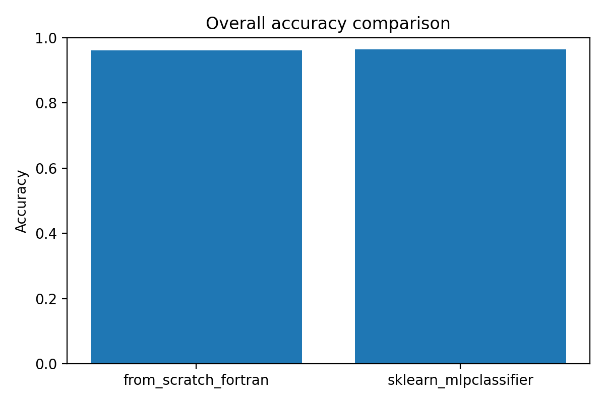
| Model | Accuracy |
|---|---|
| From-scratch Fortran | 96.15% |
| scikit-learn MLP | 96.35% |
The gap is 0.2 percentage points. That's smaller than I expected.
Scikit-learn has advantages I didn't implement: adaptive learning rates (Adam), regularization, smarter weight initialization. The fact that vanilla gradient descent gets within 0.2% suggests the core algorithm is sound.
What the Confusion Matrix Revealed
The confusion matrix shows where the model succeeds and where it struggles:
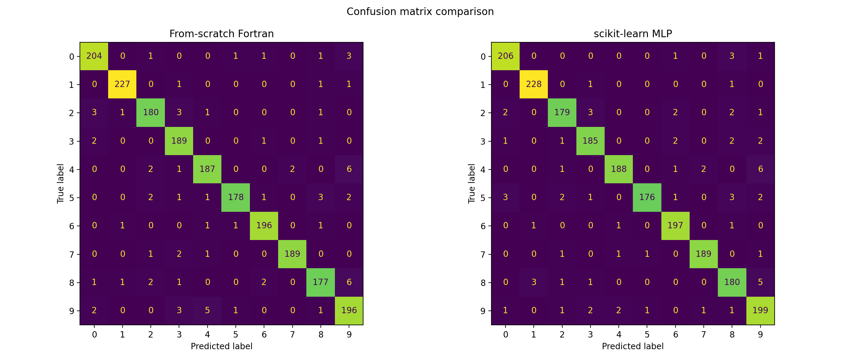
Both models show similar error patterns. The from-scratch model confuses 4s and 9s — they share similar stroke structures. It struggles with 3s and 8s for the same reason. These aren't bugs in the implementation; they're limitations of a single-hidden-layer network on raw pixel features.
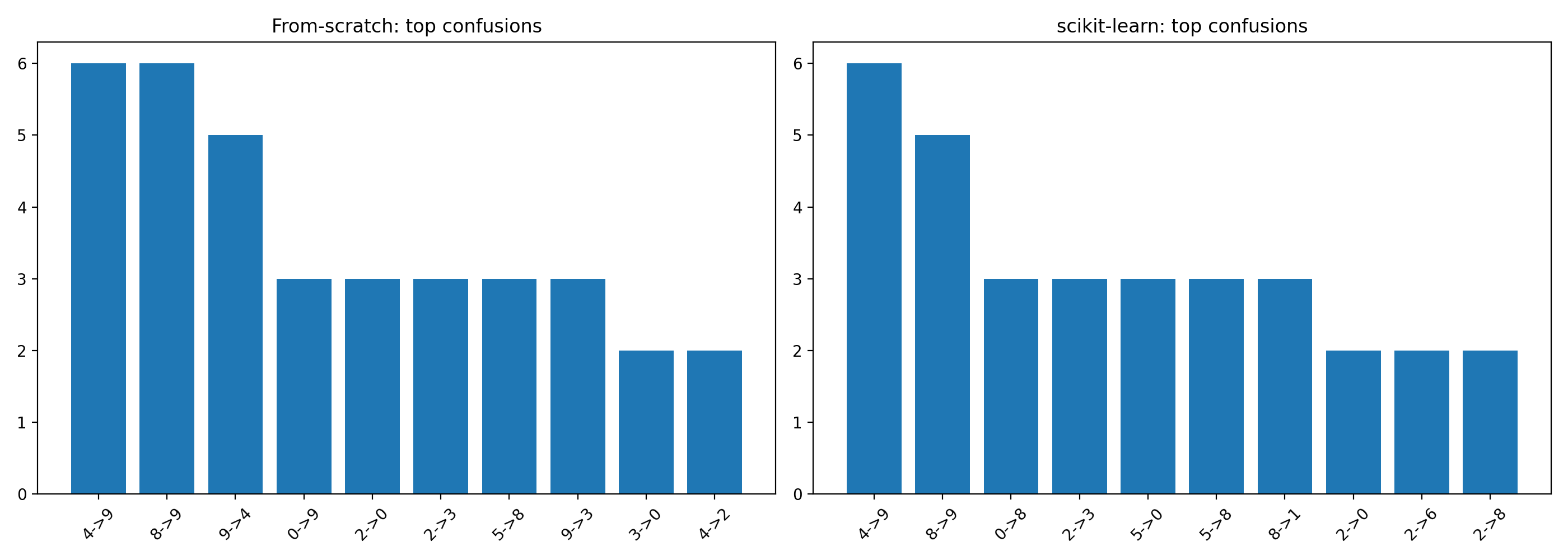
The top confusion pairs are nearly identical between the two models, which further validates that the from-scratch implementation is learning the same patterns as the optimized library.
Per-Class Performance
Breaking down performance by digit class reveals where each model excels:
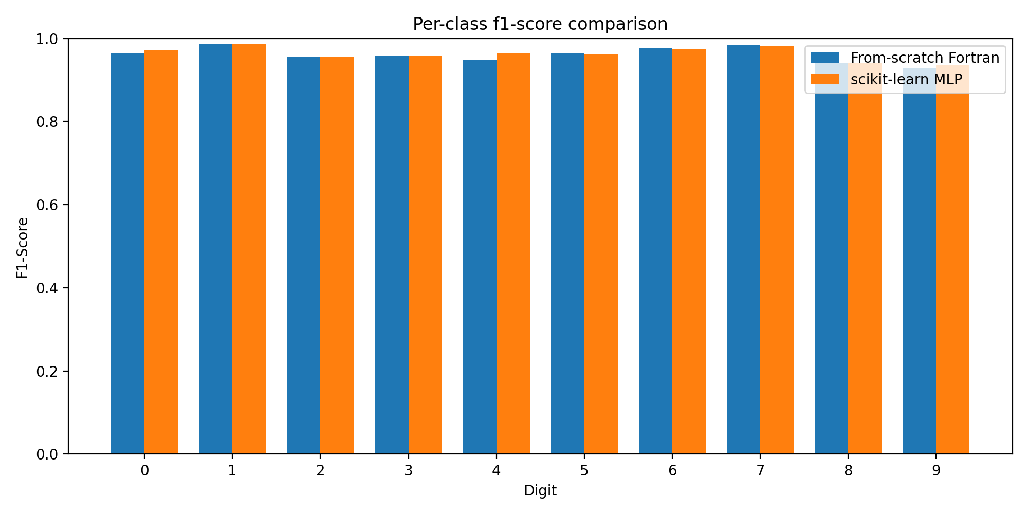
The F1 scores are remarkably close across all 10 classes. Some digits (like 0 and 1) are easy for both models. Others (like 8 and 9) show slightly lower performance — these are the digits with more variation in handwriting style.
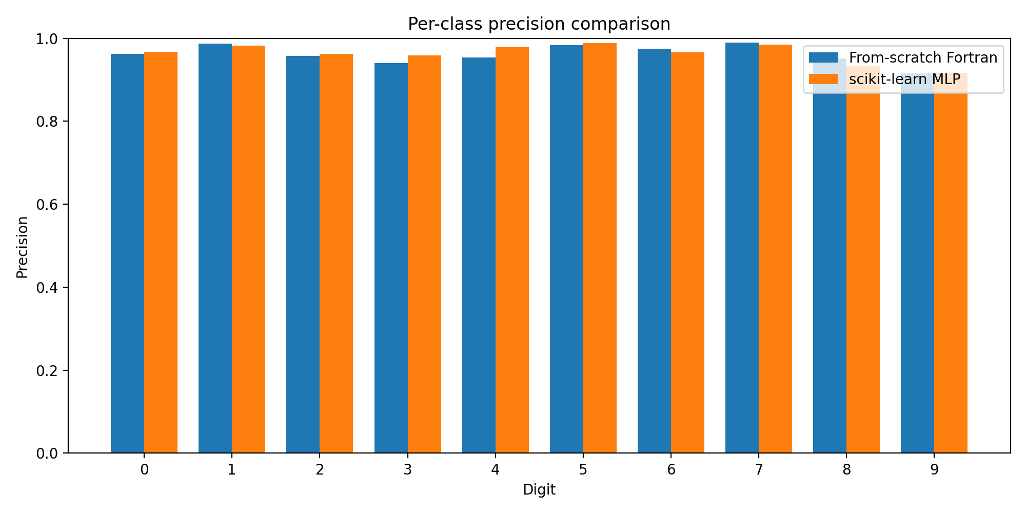
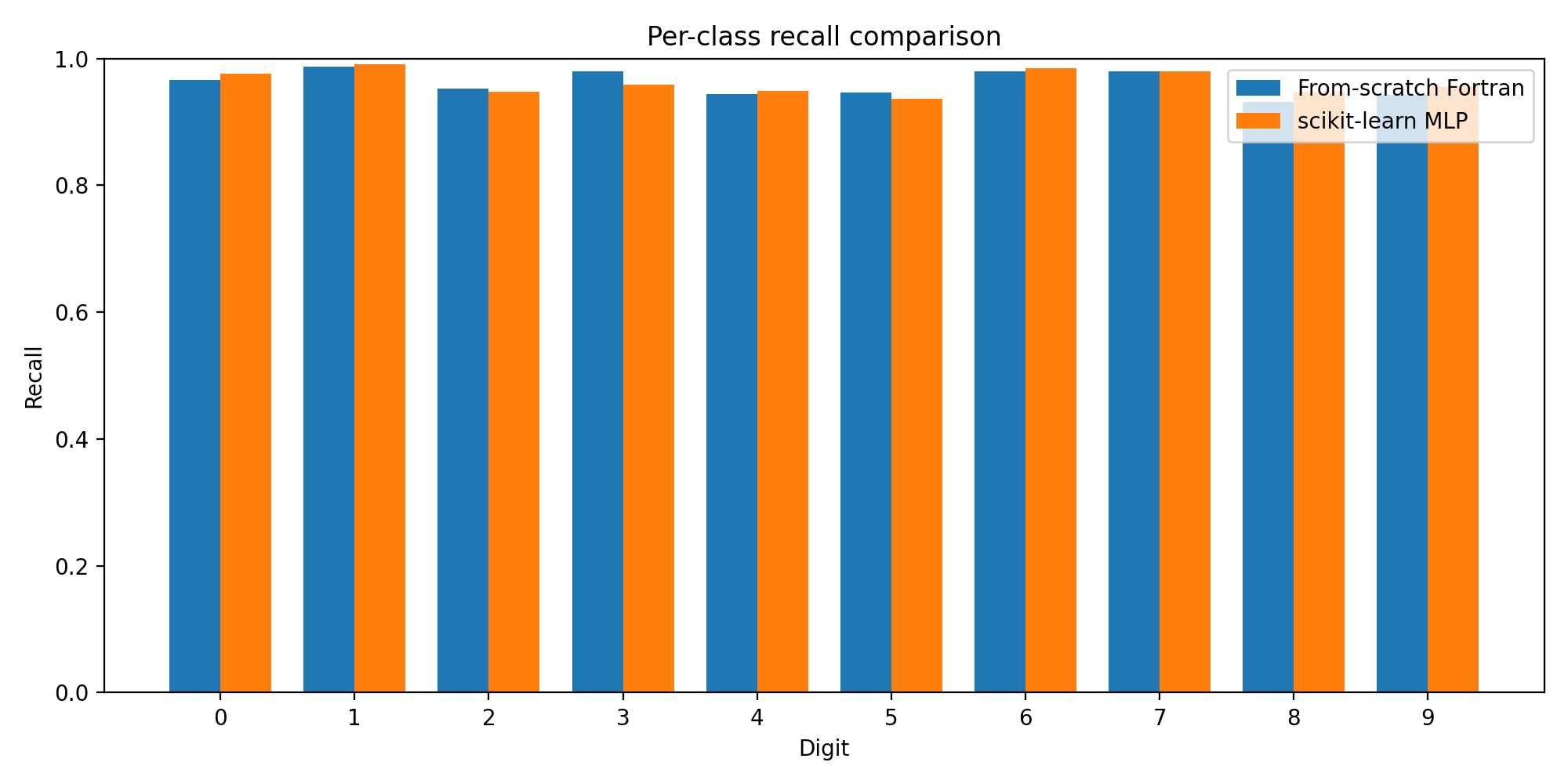
The precision and recall charts tell the same story: the from-scratch model tracks the scikit-learn baseline almost exactly, class by class.
Error Analysis
Looking at actual misclassifications helps understand what the model finds difficult:
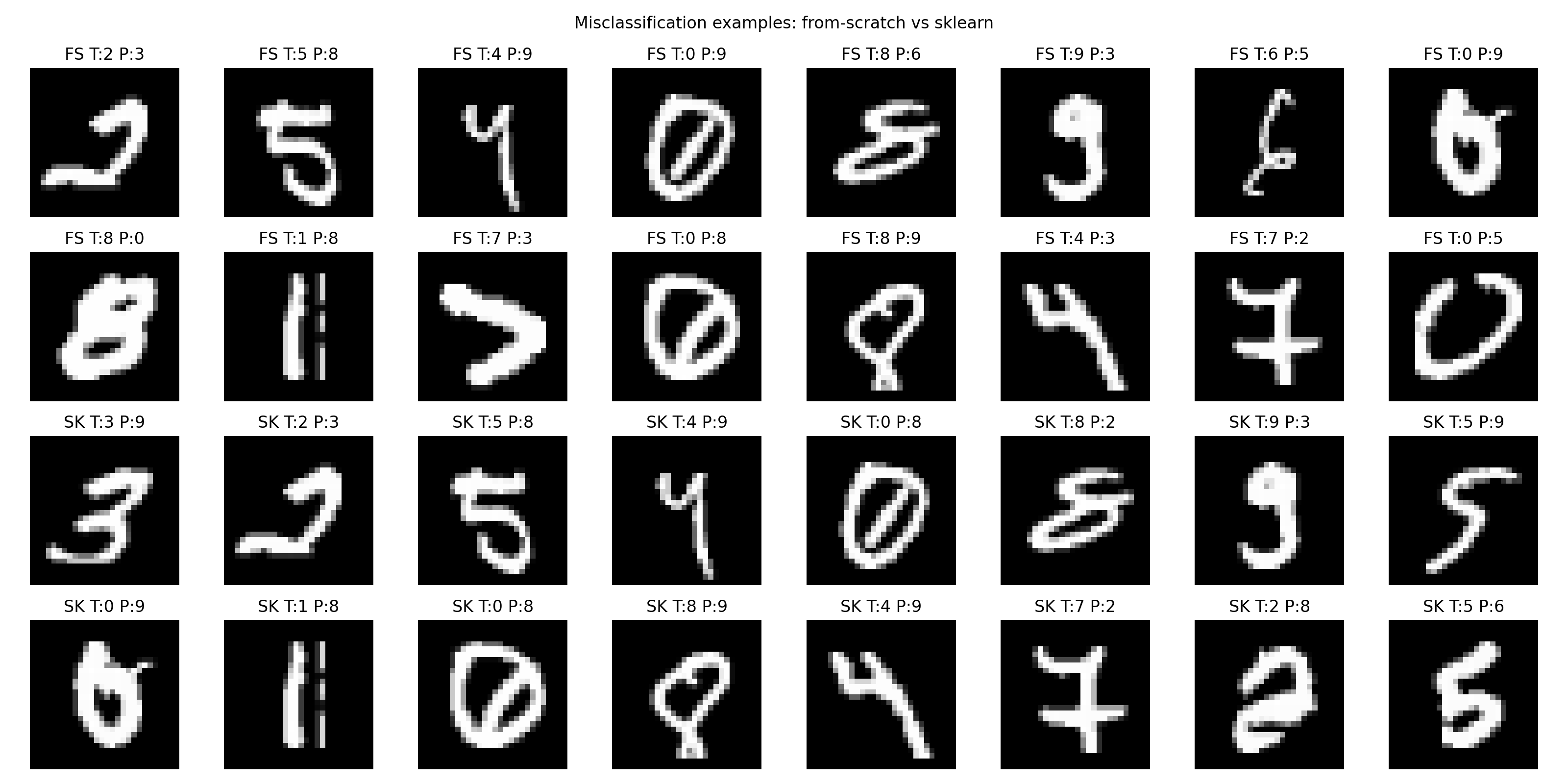
Many of the errors are ambiguous even to humans — digits written sloppily, or in unusual styles. When the model fails, it's often on cases where the "correct" label is debatable.
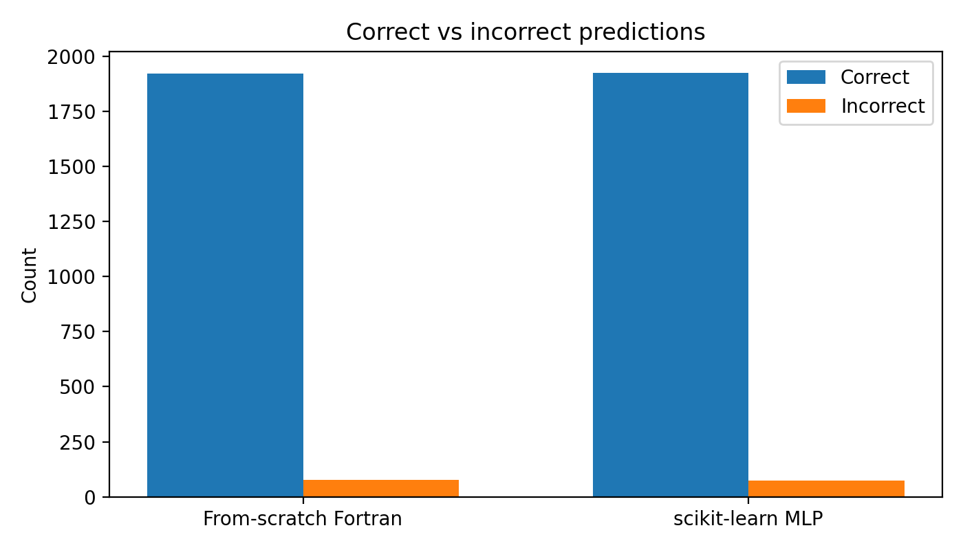
The overall correct/incorrect split is nearly identical between models. The from-scratch implementation isn't systematically worse — it's making the same kinds of mistakes on the same kinds of inputs.
What I Learned
Loss function choice matters more than architecture tweaks. Switching from MSE to cross-entropy had a bigger impact than doubling the hidden layer size.
Numerical stability is invisible until it isn't. The softmax overflow issue cost me an evening. Frameworks handle this automatically; from-scratch implementations don't.
Manual backprop forces you to understand the math. When training diverges, you can't just Google the error message. You have to trace through the gradient computation and find the bug.
Fortran is surprisingly pleasant for numerical code. Array slicing, column-major storage, and mature compilers make matrix operations clean. The language has aged, but the core design holds up.
What's Next
The current model is intentionally simple. Potential extensions:
- Mini-batch gradient descent — reduce memory usage and enable stochastic dynamics
- Momentum or Adam — implement adaptive learning rates from scratch
- Deeper architectures — add a second hidden layer, manually derive the gradients
- Convolutional layers — the real test of from-scratch implementation
- GPU acceleration — explore CUDA Fortran or OpenACC
But the main goal is already achieved: I now understand what happens inside a neural network, not because I read about it, but because I built it.
The Code
The full implementation is open source:
src/nn/serial_nn_multiclass.f90— the neural network modulesrc/nn/run_serial_nn_multiclass_realdata.f90— the training driverscripts/— Python evaluation and visualization toolsexperiments/— hyperparameter configurationsresults/figures/— all visualizations shown above
View the repository on GitHub →
If you're interested in scientific computing, numerical programming, or ML from first principles, I'd be happy to discuss. Reach out through the contact form or connect on LinkedIn.
Comments