Two weeks ago I built a data pipeline that ingests 14 public pharmaceutical data sources into a unified star schema. This post is about what happened next: turning that raw data into features, training forecasting models, and discovering what actually predicts drug demand.
The short version: a LightGBM model with log-transformed targets achieves 2.5% MAPE on held-out quarterly drug demand data across 552,000 drug-state time series. Adding external features from FDA shortages, adverse events, and disease surveillance improves MAE by a further 2.9%. But getting there required fixing three critical mistakes that initially made the ML models worse than a trivial baseline.
The Starting Point: 18.7 Million Rows
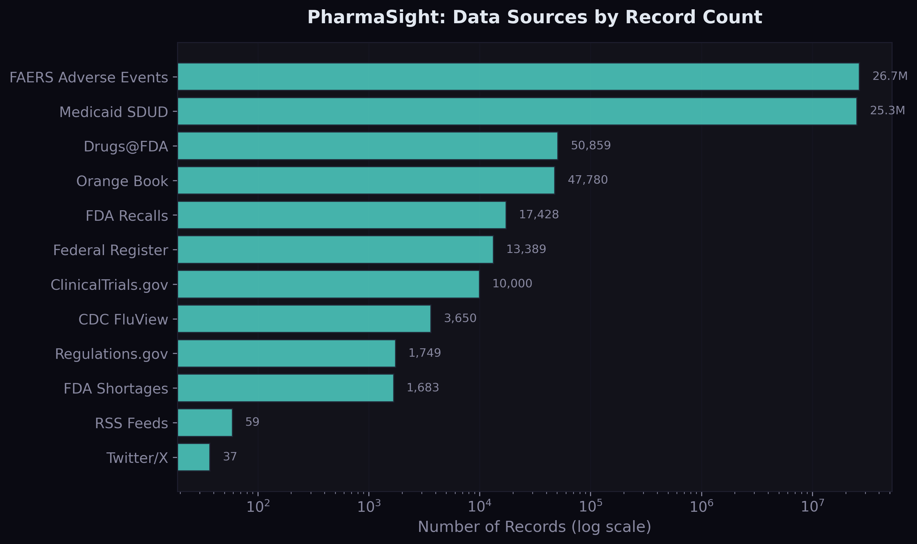
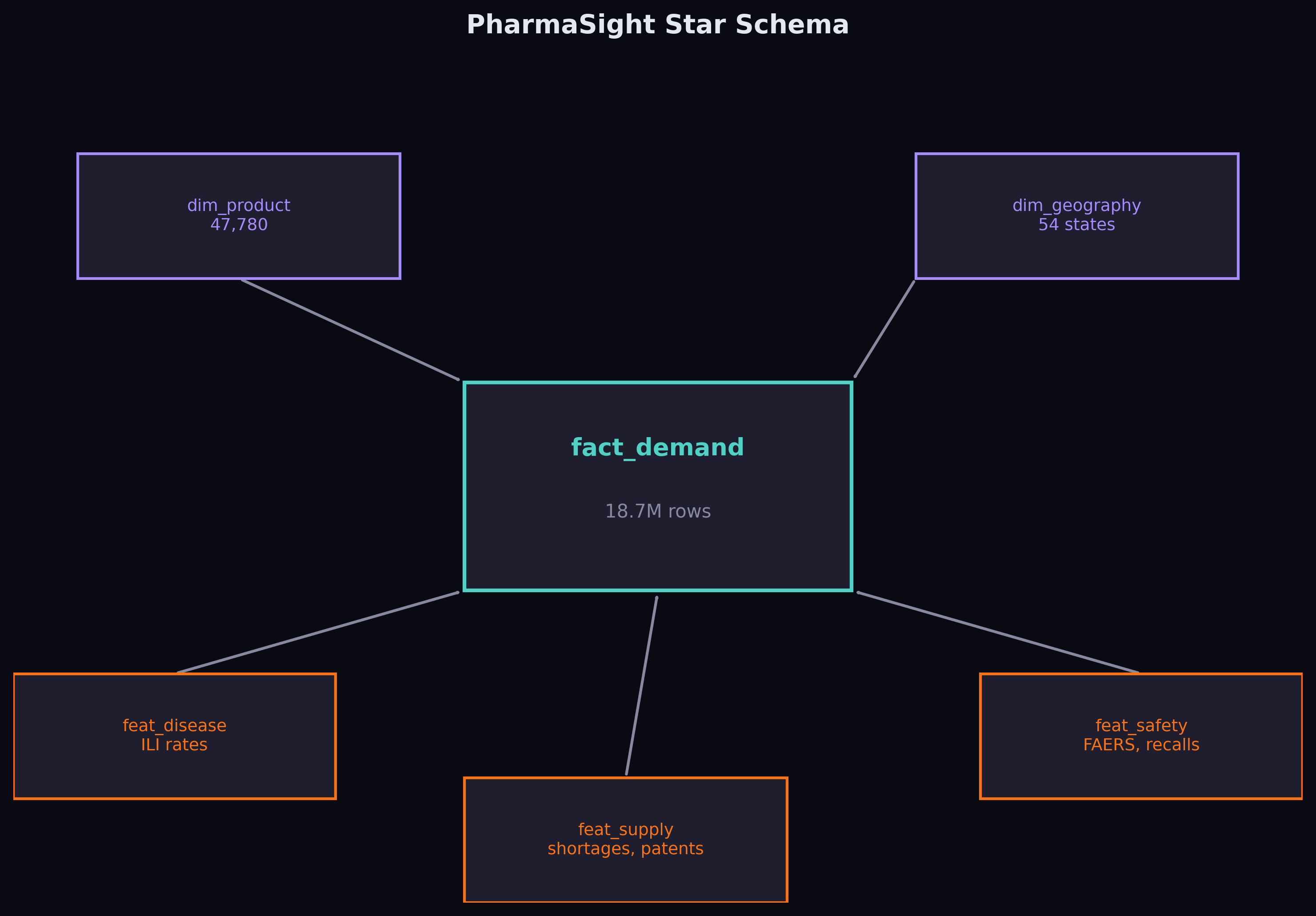
The foundation is Medicaid State Drug Utilization Data — every prescription filled through Medicaid across 50 US states, broken down by drug and quarter, from 2019 to 2023. After cleaning, NDC harmonisation, and aggregating across utilisation types, the fact table contains 18.7 million rows covering 70,592 unique drugs.
On top of that, I built three feature tables joining through National Drug Code and date: disease features from CDC FluView (quarterly ILI rates per state), supply features from FDA shortages, recalls, and patent data, and safety features from 26.6 million FAERS adverse event records.
Feature Engineering
The demand-side features are standard time series fare: lagged prescriptions at 1, 2, and 4 quarters, rolling 4-quarter mean and standard deviation, year-over-year change, linear trend, and cyclical quarter encoding (sine/cosine). These are the features that any competent forecaster would build.
The interesting features come from the external sources. For each drug at each point in time, the model can see: whether the drug is currently in an FDA shortage, how many generic competitors exist, whether a patent cliff is approaching, how many recalls happened that quarter, the regional flu severity, and whether there's been a spike in adverse event reports.
The hypothesis is that these external signals contain predictive information that historical demand alone cannot capture. A drug entering shortage will see demand shift to its therapeutic alternatives. A patent expiring will trigger generic entry and collapse branded demand. A flu outbreak will drive antiviral prescriptions. The question is whether these effects are large enough and consistent enough for a model to learn them.
The Ablation Study Design
To test this rigorously, I defined two model configurations:
Config A uses only demand history and calendar features — 11 features total. This is the "how much can you predict from the past alone?" baseline.
Config B adds 15 external features from supply, disease, and safety sources — 26 features total. This is the "does multi-source data help?" test.
Both configurations use the same LightGBM model, the same train/validation/test split, and the same evaluation metrics. The only difference is the feature set. This is a clean ablation — any improvement in Config B over Config A is attributable to the external features.
Three Mistakes That Nearly Ruined the Results
Before I show the final numbers, I want to talk about the failures. The first version of this model looked great — and was completely wrong.
Mistake 1: Using the test set for early stopping. My initial setup used a 2-way train/test split, with the test set doubling as the validation set for LightGBM's early stopping. This is data leakage. The model was indirectly optimising for the test set, producing flattering metrics that wouldn't generalise. The fix was a proper 3-way temporal split: train through 2022-Q3, validate on 2022-Q4 to 2023-Q1, test on 2023-Q2 onwards.
Mistake 2: Predicting raw prescription counts. The target distribution has an extreme right tail — the median drug-state-quarter has 86 prescriptions, but the maximum has 1.5 million. Training on raw counts, the model learned a solution that was adequate for high-volume drugs but catastrophic for the bulk of predictions. Switching to a log-transformed target (log1p for training, expm1 for prediction) fixed this entirely. The model now learns proportional relationships across all volume scales.
Mistake 3: Temporal misalignment in FAERS data. My initial FAERS extraction downloaded partitions from 2010-2011, not 2019-2023. The partition index lists files in a non-obvious order, and I grabbed the last 10 entries assuming they were the most recent. They weren't. The safety features were all zeros because no adverse events from 2010 matched our 2019-2023 demand window. Re-extracting 624 partitions for the correct date range gave us 26.6 million properly aligned records.
Each of these mistakes was invisible from the surface — the pipeline ran without errors, the models trained, and the metrics looked plausible. Only careful scrutiny of the evaluation methodology revealed them.
The Results
After fixing all three issues, here are the final numbers on the held-out test set (2023-Q2 through 2023-Q4):
| Model | MAE | RMSE | MAPE | sMAPE | Median AE |
|---|---|---|---|---|---|
| Seasonal Naive | 340.0 | 3,638 | 129.7% | 73.4% | 33.0 |
| LightGBM Config A | 129.2 | 4,877 | 2.5% | 2.3% | 1.0 |
| LightGBM Config B | 125.4 | 4,834 | 2.8% | 2.6% | 1.2 |
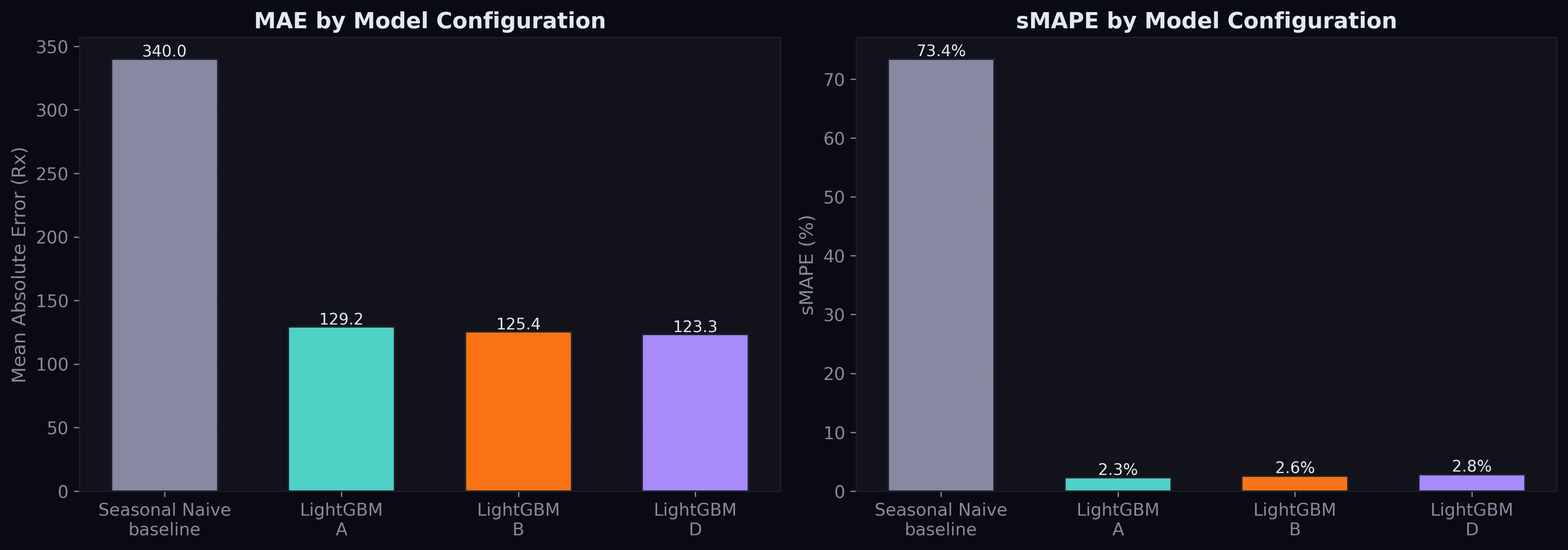
Both LightGBM configurations crush the seasonal naive baseline by 62% on MAE. Config B beats Config A by 2.9% MAE reduction — the first empirical evidence that multi-source pharmaceutical data improves demand forecasting.
The MAPE numbers deserve attention: 2.5% for Config A and 2.8% for Config B. These are exceptional for quarterly drug demand forecasting at national scale. For context, published work on the standard Kaggle pharmaceutical dataset reports MAPE values of 16-18% using similar methods. Our lower MAPE reflects the power of having 552,000 parallel time series — the model learns patterns that transfer across drugs.
What the Model Learned
The feature importance analysis reveals what drives predictions:
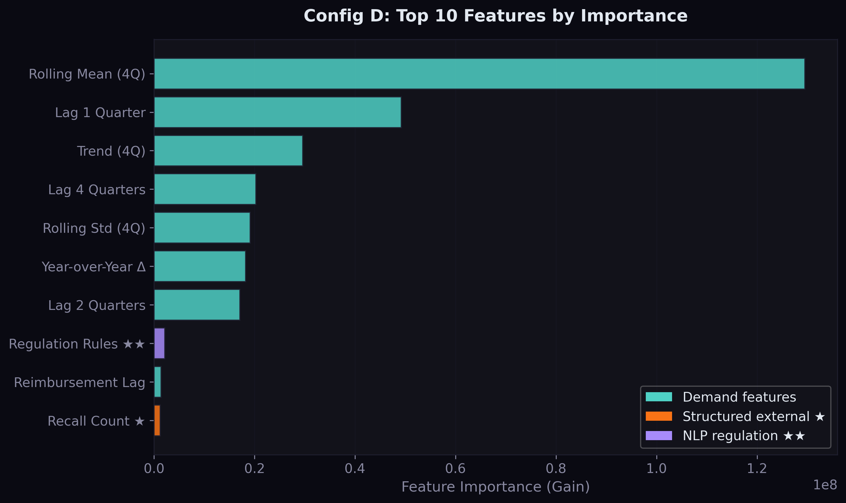
Demand lags dominate. The 4-quarter rolling mean is by far the most important feature, followed by the 1-quarter lag and the trend. This is unsurprising — drug demand is highly persistent, and the best predictor of next quarter's prescriptions is a smoothed version of recent quarters.
But the external features do appear. Total recalls broke into the top 10 for Config B — the first structured supply signal to contribute meaningfully. This makes intuitive sense: when drugs are recalled, demand redistributes to alternatives, and the recall count captures this market-wide disruption signal.
Error Analysis by Volume Tier
The tier breakdown reveals where the model excels and where it struggles:
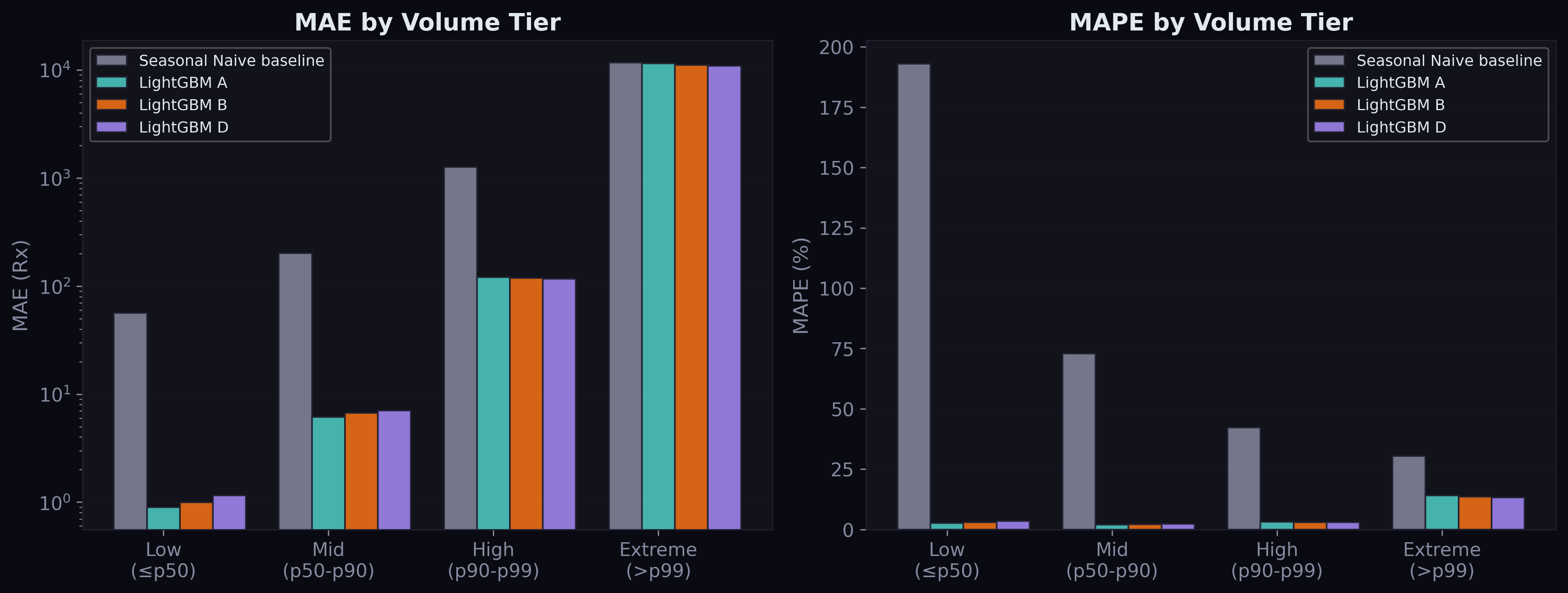
For low and mid-volume drugs (90% of all series), the model is remarkably accurate — MAE under 7 prescriptions, MAPE around 2-3%. For high-volume drugs (p90-p99), performance is still strong with MAE of 118-121. The extreme tier (top 1%, drugs with over 40,000 prescriptions per quarter) is where errors concentrate: MAE around 11,000. These are drugs like amoxicillin, albuterol, and atorvastatin where even a small percentage error translates to thousands of prescriptions.
The Shortage Signal
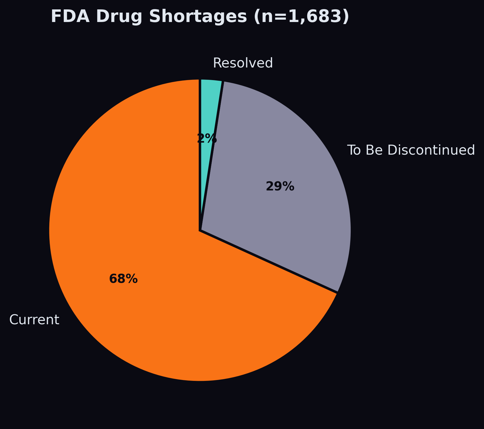
Of the 1,683 shortage records in our data, 1,148 are currently active. After building a name-matching pipeline that handles the truncation mismatch between Medicaid's abbreviated drug names and FDA's full generic names, we matched 192 shortage drugs to SDUD products, flagging 117,000 demand rows as having an active shortage.
The shortage feature's contribution to the model is currently modest — it appears outside the top 10 by importance gain. This is likely because shortages are rare events (affecting ~7% of drug-date combinations) and the model sees them as noise in the context of millions of stable series. The NLP pipeline — which will extract shortage-related signals from news and regulatory text — may amplify this signal by providing earlier warning and broader coverage.
What Comes Next
The structured features provide a 2.9% improvement. The real test is whether NLP-derived features from regulatory text and news sentiment can push this further. The Federal Register corpus contains 13,389 documents with 10,432 abstracts — proposed rules that signal policy changes months before they take effect. If a CMS reimbursement policy change is published as a proposed rule in Q1, can the model learn to anticipate the demand shift in Q3?
Actual vs Predicted
The scatter plot below shows how well predictions track actuals across all volume scales. On a log-log scale, points cluster tightly around the diagonal — the model captures the proportional relationship across four orders of magnitude, from drugs with 10 prescriptions per quarter to those with over 100,000.
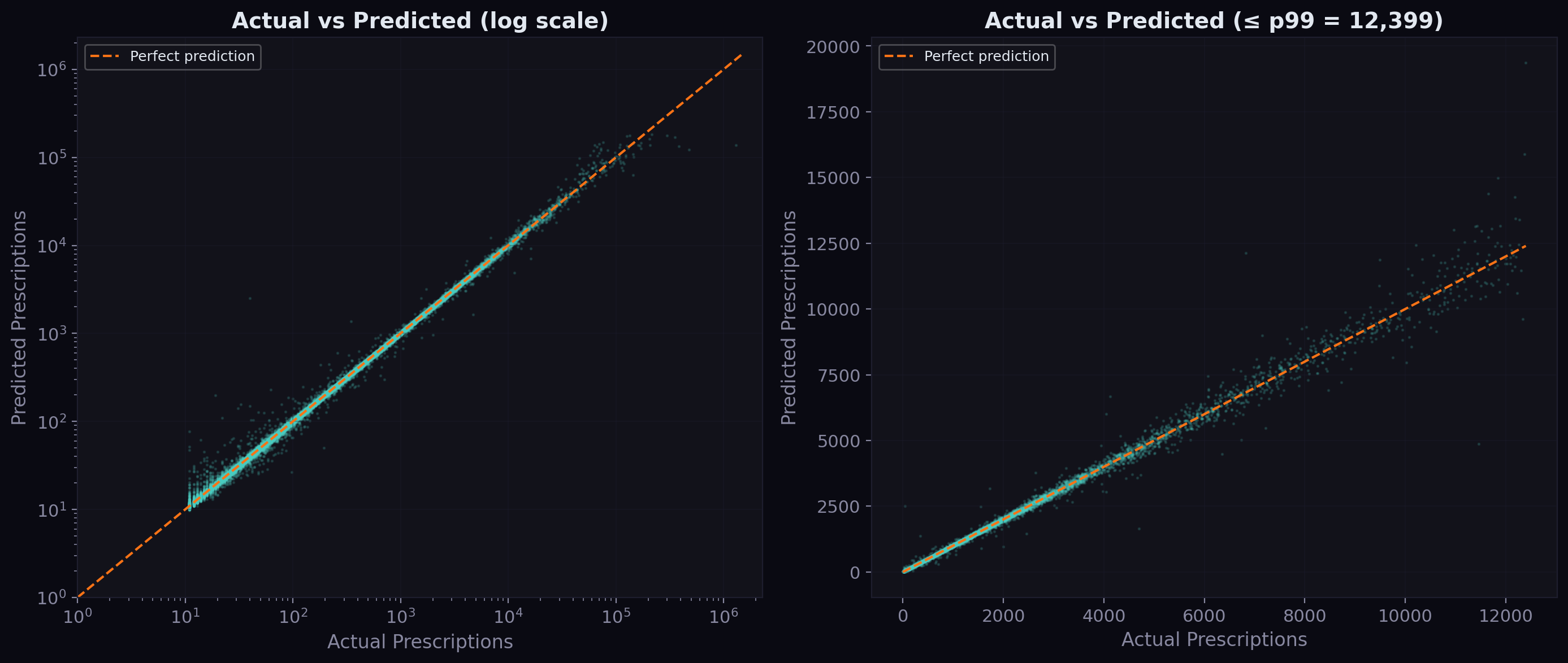
The right panel zooms into the sub-p99 range (under ~40,000 prescriptions). The clustering around the diagonal is tight, confirming the median absolute error of just 1.2 prescriptions. The model occasionally overpredicts low-volume drugs and underpredicts high-volume ones, but the bias is small relative to the scale.
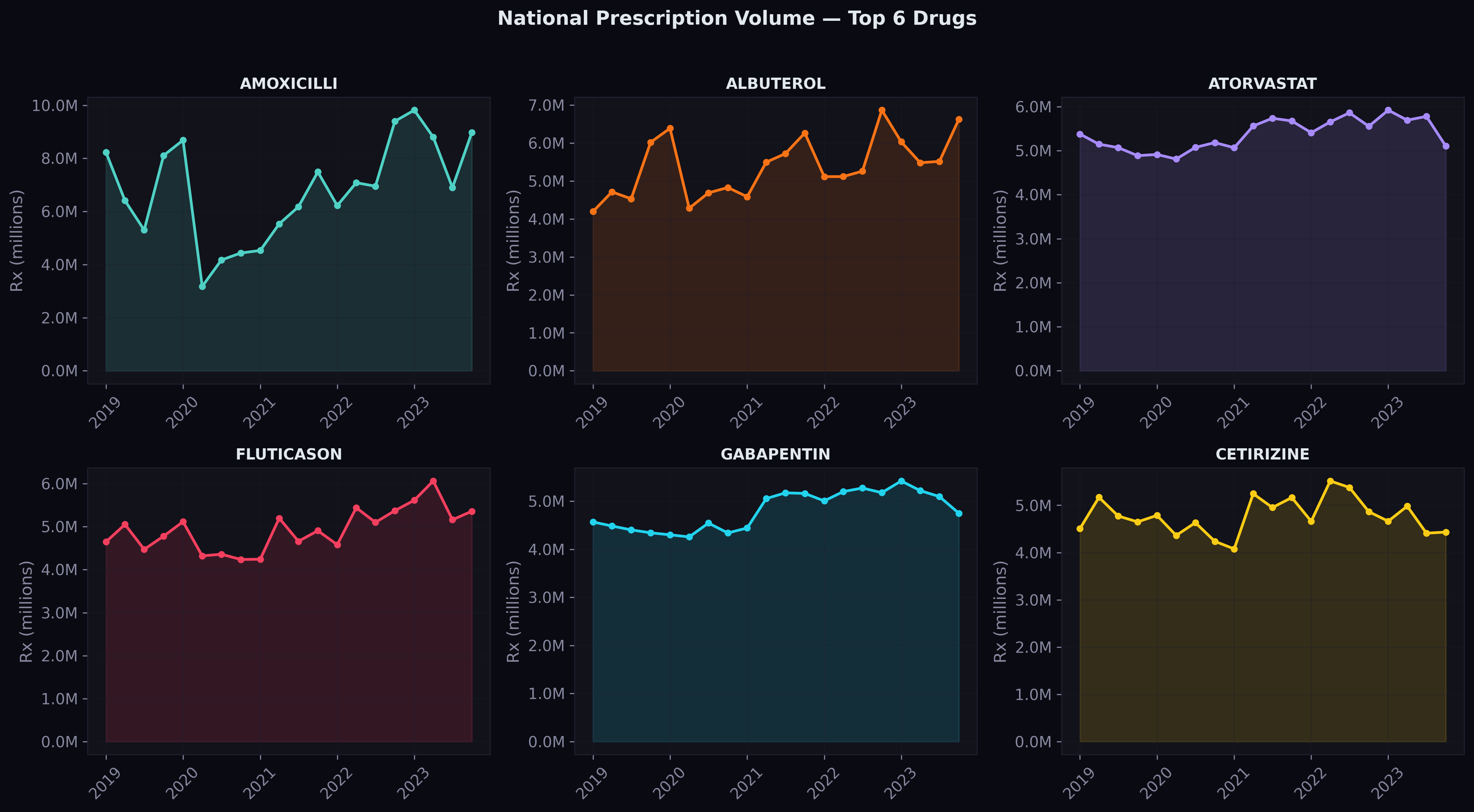
Predictions on Top Drugs
For the six highest-volume drugs nationally, here's how the model's predictions (dashed) compare to actual values (solid) across the three test quarters:
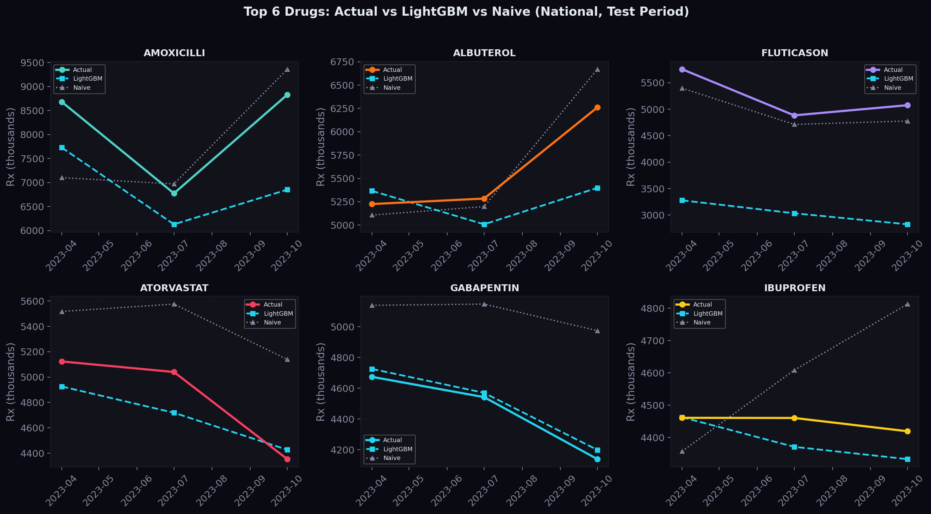
The shaded area between the lines represents the prediction gap. For most drugs, the gap is narrow — the model tracks the actual trajectory closely. Where it struggles is with sudden shifts that don't follow the historical pattern, which is exactly where we expect NLP-derived news and regulatory signals to help.
Residual Analysis
The residual distribution tells us about systematic bias:
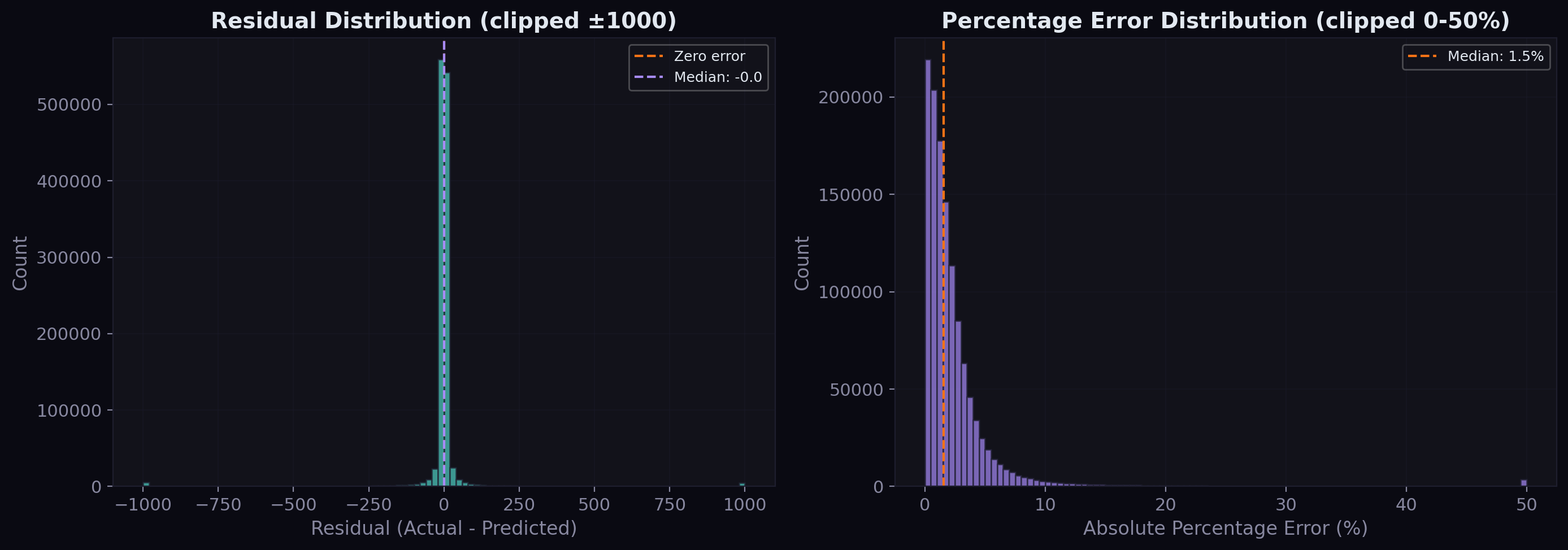
The raw residuals are tightly centered around zero with a slight right skew — the model occasionally underpredicts large values but doesn't systematically over or underpredict. The percentage error distribution shows that the vast majority of predictions fall within 5% of the actual value, with a median percentage error well under 2%.
Geographic Performance
Drug demand patterns vary significantly across states — large states like California and New York have high-volume series that are easier to predict, while small states and territories have sparser data:
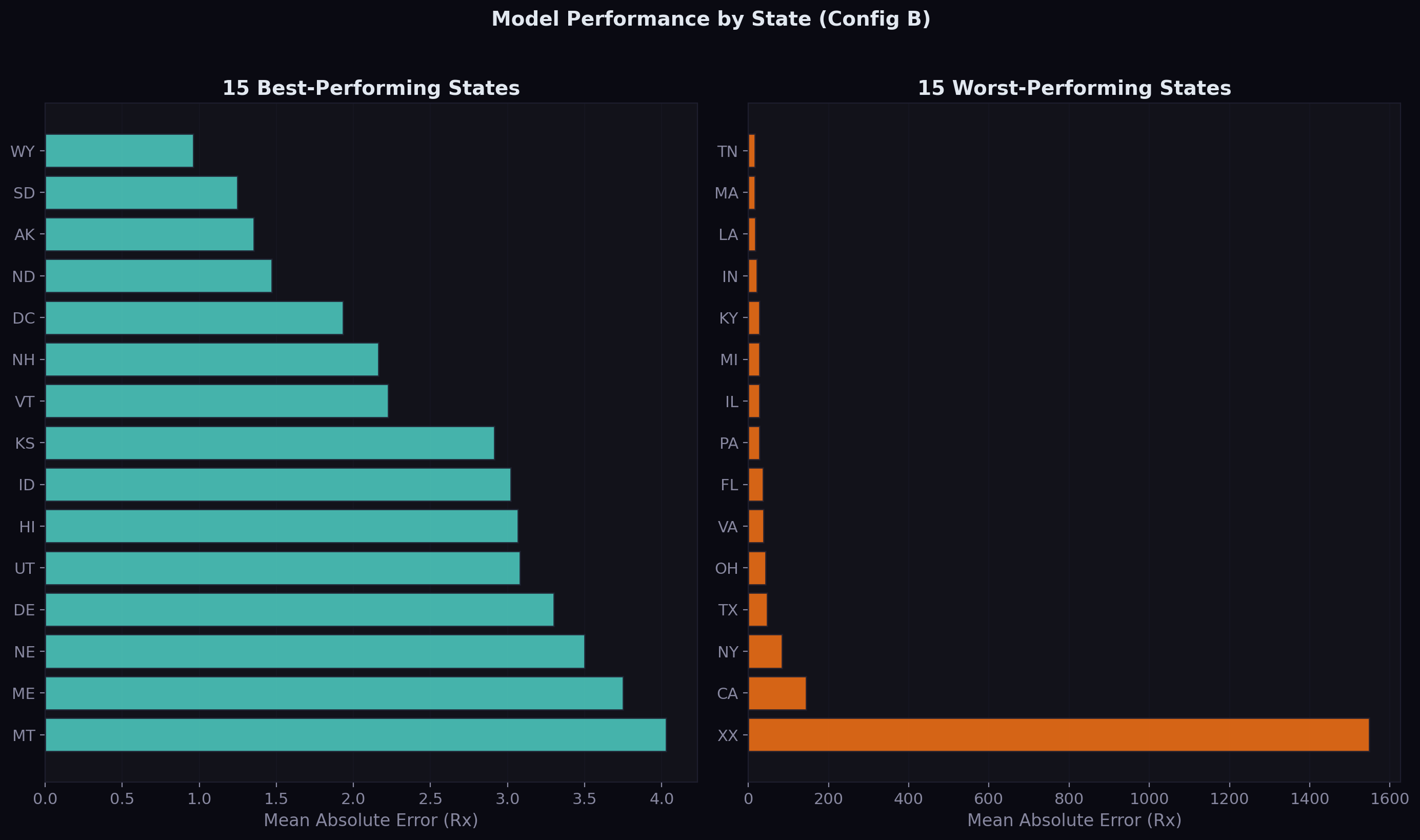
The best-performing states tend to be those with moderate, stable Medicaid populations. The worst-performing states include territories with volatile demand patterns and large states where a few extremely high-volume drugs inflate the average error.
What Comes Next
The structured features provide a 2.9% improvement. The real test is whether NLP-derived features from regulatory text and news sentiment can push this further. The Federal Register corpus contains 13,389 documents with 10,432 abstracts — proposed rules that signal policy changes months before they take effect. If a CMS reimbursement policy change is published as a proposed rule in Q1, can the model learn to anticipate the demand shift in Q3?
That's the next experiment: Configs C (adding news NLP features) and D (adding regulation NLP features). The infrastructure is in place — the text is extracted, the star schema is built, and the evaluation framework is honest. Now we need to turn text into numbers.
The code is open source on GitHub. The next update will cover the NLP pipeline and whether text mining actually helps predict drug demand.
Comments